Plots of drawdown against the drawdown function is one of the methods to determine aquifer transmissivity (Shtengelov, 1994). These plots can be interpreted for aquifer transmissivity based on the slope of a straight line. Axis Y corresponds to factual drawdown measurements, while axis X presents the function f(.) values that are calculated by different equations for different drawdown solutions. These solutions include hydraulic diffusivity and may include leakage factor.
This method can be accessed through the menu "Analysis > Drawdown - function".
The plots are prepared based on the last input (or determined by other methods) parameters. Parameters can be changed through the menu "Analysis > Direct solution" or by clicking the right mouse button on the left bottom corner of the plot window. The shape of the plot should be independent of input transmissivity and the line should start at the coordinate origin. Transmissivity is determined by the slope of the straight line.
Interpretation can be conducted by plotting data from all observation wells on the same plot. In ideal interpretation all points will be plotted along the same line.
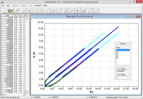
Example of determination aquifer transmissivity using the s-f(.) plot for infinite confined aquifer. When theoretical hydraulic diffusivity is smaller than its real value, the function f(.) is smaller as well and, therefore, the points are located along the line that is above the straight line from the coordinates origin
This method can be applied for the Theis method and for leaky aquifers with constant head in the adjacent aquifer. Other limitations are that only one pumping well with constant pumping rate is allowed and the aquifer must be isotropic.
Straight line shape of plots results from the linear structure of drawdown solutions. For example, for the Theis's solution:
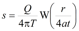
The plots are prepared for axes:
![]()
where
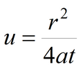
and slope of the straight line is:
![]()
The transmissivity of the aquifer is determined from the above equation.
When hydraulic diffusivity is correctly determined, the plotted straight line will start at the coordinates origin.
For steady state conditions (for example, pumping near a constant-head boundary), steady state intervals are not dependent on hydraulic diffusivity and, therefore, can't be interpreted. All measurement in state conditions will be plotted on the single plot. In this case, transmissivity can only be determined on the interval between the coordinates origin and start of the steady state regime.
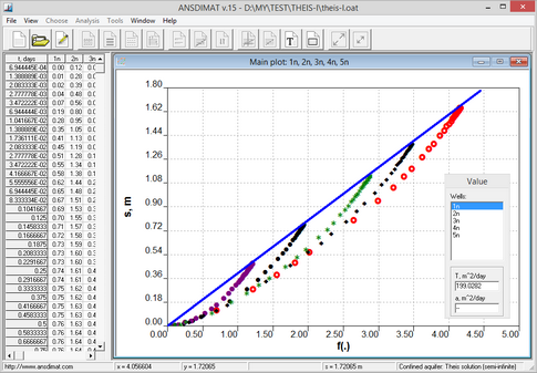
Example of interpretation using s – f(.) plot for a pumping test with five observation boreholes in a confined constant-head bounded aquifer. Prior to steady state regime the measurements deviate from the straight line because of incorrectly determined hydraulic diffusivity.
References
Shtengelov, 1994. Hydrodynamic simulations on computer (In Russian: Гидродинамические расчеты на ЭВМ / Под ред. Р.С. Штенгелова. М.: Изд-во МГУ, 1994).